Overview
When analysing citizen science data, it is often necessary to
restrict your dataset to a specific geographic area. obsR
provides two primary ways to achieve this within the
obs_read() function:
-
bbox: A simple rectangular bounding box defined asc(xmin, ymin, xmax, ymax)in longitude and latitude. -
polygon: A precise geographic area (e.g., a protected site, a municipality, or a custom study plot). Points must fall strictly inside the polygon, not just within its bounding box.
(Note: Language and label handling is covered in a separate
vignette: vignette("labels")).
library(obsR)
db <- obs_example_db()
Defining a Polygon Area
The polygon argument is highly flexible and accepts
several formats. All polygon operations require the sf
package to be installed.
You can provide the area as: 1. A WKT string
(POLYGON or MULTIPOLYGON). 2. A
GeoJSON string (a Polygon,
Feature, or FeatureCollection). 3. A
file path to a local .geojson,
.json, or .wkt file. 4. An existing
sf or sfc polygon object.
Example 1: Using a WKT String
# Define a simple rectangular park boundary (xmin, ymin, xmax, ymax)
park_wkt <- "POLYGON ((-6.1 37.3, -5.8 37.3, -5.8 37.5, -6.1 37.5, -6.1 37.3))"

# Filter observations strictly inside this polygon
inside_park <- obs_read(db, polygon = park_wkt)

nrow(inside_park)
#> [1] 438
range(inside_park$lng)
#> [1] -6.094748 -5.817471
range(inside_park$lat)
#> [1] 37.3026 37.4827
Example 2: Combining Spatial and Attribute Filters
Spatial filters can be seamlessly combined with standard attribute
filters (like species or date). obsR applies species and
date filters first, then the spatial filter, and finally any
limit you have set.
house_in_park <- obs_read(
  db,
  species = "Passer domesticus",
  date = c("2020-01-01", "2020-12-31"),
  polygon = park_wkt
)

nrow(house_in_park)
#> [1] 425
If the defined area contains no data, obs_read() will
safely return zero rows without throwing an error:
Example 3: GeoJSON, Files, and sf Objects
The same area can be defined using GeoJSON. Coordinates must always
be in [longitude, latitude] order.
park_gj <- '{"type":"Polygon","coordinates":[[[-6.1,37.3],[-5.8,37.3],[-5.8,37.5],[-6.1,37.5],[-6.1,37.3]]]}'

# Both methods yield the exact same observation IDs
identical(
  obs_read(db, polygon = park_wkt)$id,
  obs_read(db, polygon = park_gj)$id
)
#> [1] TRUE
For recurring analyses, it is often more practical to load a boundary
from a file or use an sf object you have already
prepared:
# 1. From a local file
gj_file <- tempfile(fileext = ".geojson")
writeLines(park_gj, gj_file)
from_file <- obs_read(db, polygon = gj_file)

# 2. From an sf object
poly_sf <- sf::st_as_sfc(park_wkt, crs = 4326)
from_sf <- obs_read(db, polygon = poly_sf)

# Both work identically to the string methods
nrow(from_file)
#> [1] 438
nrow(from_sf)
#> [1] 438
(Note: The polygon argument works identically for
CSV and Excel exports).
Coordinates and CRS Alignment
obsR expects all coordinates (lng and
lat) to be in the WGS84 coordinate reference system
(EPSG:4326).
obsR does not perform geocoding (e.g., looking up
municipalities by name). You must provide the spatial boundary yourself.
If you are joining the resulting data with another spatial layer, ensure
the CRS matches first:
# 1. Load data and convert to sf object
obs <- obs_read(db)
obs_sf <- sf::st_as_sf(obs, coords = c("lng", "lat"), crs = 4326, remove = FALSE)

# 2. Ensure your boundary layer is also in EPSG:4326
park_sf <- sf::st_sf(geometry = sf::st_as_sfc(park_wkt, crs = 4326))
# If your layer was in a different CRS, transform it first:
# park_sf <- sf::st_transform(park_sf, 4326)

# 3. Perform the spatial join
joined <- sf::st_join(obs_sf, park_sf, left = FALSE)
nrow(joined)
#> [1] 438
Visualising the Filtered Area
You can draw the boundary of your polygon directly on the map using
obs_map(polygon = ...).
- If
datainobs_map()is a file path, the function will both filter the points and draw the boundary. - If
datais already anobs_df(a loaded dataset), it will only draw the boundary. In this case, you must filter the data first usingobs_read()if you want the map to reflect the spatial subset.
obs_map(inside_park, polygon = park_wkt, color = "scientific_name", basemap = "outline")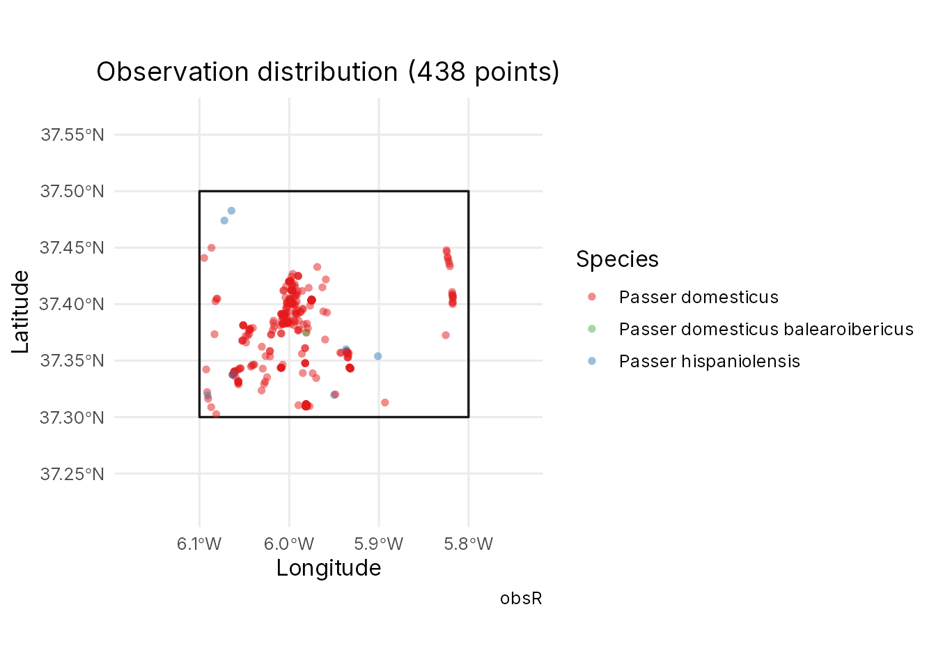
Performance Considerations
-
Memory Collection: When a
polygonfilter is applied, the data is always collected into memory. -
SQLite Limitations: Because SQLite lacks a native
spatial index,
obsRoptimises the query by first applying the polygon’s bounding box at the SQL level, and then performing the precise point-in-polygon test in R. -
Overrides: Due to this two-step process, setting
collect = FALSEor relying on row thresholds is ignored when apolygonis active. -
Combined Efficiency: You can use
bboxandpolygontogether.obsRwill intersect the rectangle with the polygon’s bounding box first, reducing the initial SQL query size before the precise polygon test runs on the remaining records.