Introduction
obsR is designed to read and analyse data
exports (SQLite, CSV, or Excel) that you have already
obtained from Observation.org.
Important: obsR is not a
client for the live Observation.org API. obsR focuses
exclusively on transforming bulk export files into clean, analysis-ready
data frames. You do not need to write SQL queries or memorise the
intricacies of the export schema; the package handles the
standardisation of columns, validation statuses, phenology, and
more.
Reading Your Data
The obs_read() function is your entry point. Below, we
use an example dataset of House Sparrow and Spanish Sparrow observations
in Seville.
library(obsR)

db <- obs_example_db()
sparrows <- obs_read(db)
Visualising Observations
Once loaded, you can immediately map or plot your data. Without a
color argument, points are rendered in a single colour. You
can easily stratify them by species or validation status.
obs_map(sparrows, color = "scientific_name", basemap = "outline")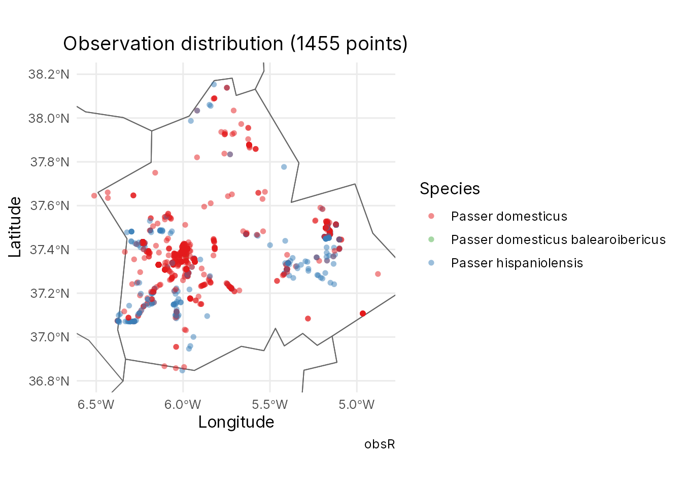
obs_map(sparrows, color = "validation", basemap = "outline")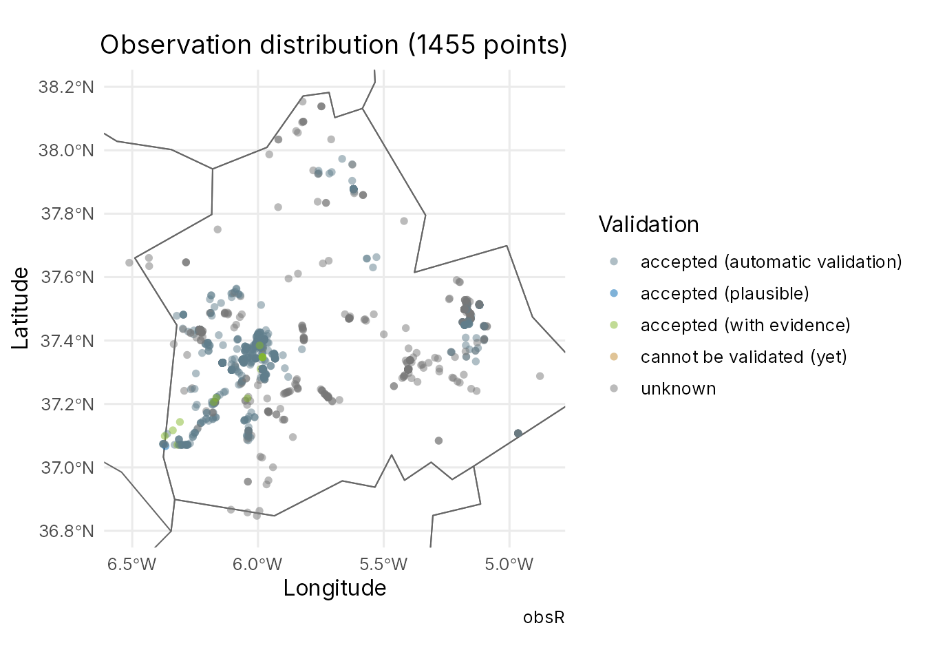
You can also generate summary plots for phenology or demographic splits:
obs_plot(sparrows, "phenology")
#> Warning: Removed 5 rows containing missing values or values outside the scale range
#> (`geom_bar()`).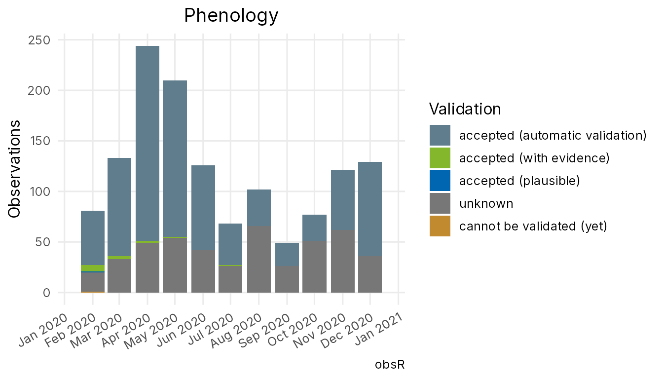
obs_plot(sparrows, "sex")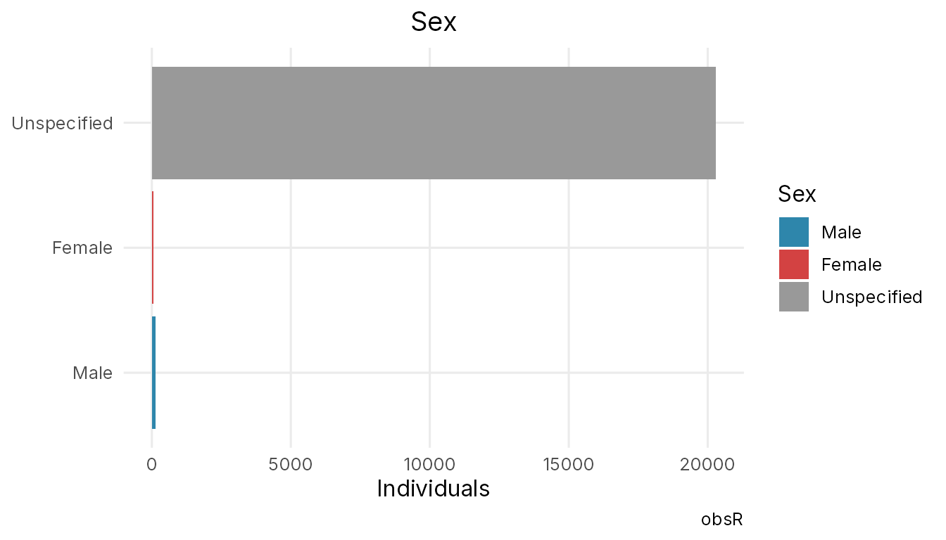
Filtering and Summarising
You can filter data directly during the import process, which is highly efficient for large SQLite files.
house <- obs_read(db, species = "Passer domesticus")
april <- obs_read(db, date = c("2020-04-01", "2020-04-30"))

obs_summary(house)
#>
#> ── Observation summary ─────────────────────────────────────────────────────────
#> Observations: 1113
#> Validated (A/J/P): 740 (66.5%)
#> Species: 2
#> Date range: 2020-01-01 to 2021-01-01
#> Multiple observations: 13
#>
#> ── Validation ──
#>
#>                       validation   n
#>  accepted (automatic validation) 729
#>                          unknown 372
#>         accepted (with evidence)  11
#>        cannot be validated (yet)   1
#> ── Sex (individuals) ──
#>          sex    n
#>  Unspecified 7579
#>         Male  125
#>       Female   67
#> ── Life stage (individuals) ──
#>      life_stage    n
#>         unknown 7274
#>           adult  468
#>  adult breeding   18
#>   second summer    7
#>        juvenile    3
#>         deviant    1
#> ── Species groups ──
#>  species_group    n
#>          Birds 1113
Handling Mixed Counts
Observation.org allows users to record a total count (e.g., “20 individuals”) while explicitly detailing the subgroup composition (e.g., “2 adult males, 5 adult females, and 13 juveniles”), specifying sex, life stage, and activity.
In SQLite exports, these mixed counts are stored as a single
row with is_multiple = TRUE and the breakdown in
the details column. - Use obs_expand() to
unpack these into individual observation rows for granular analysis
(e.g., summing individuals by sex). - Keep the compact table format for
spatial mapping. (Note: CSV and Excel exports do not currently
include this level of subgroup detail).
Data Privacy (Optional)
When sharing or publishing citizen science datasets, protecting
observer privacy is a best practice. obsR provides the
optional obs_anonymise() function to safely replace
observer names and IDs with a one-way hash.
Tip: Use a fixed salt argument if your script
needs to produce consistent anonymous codes across monthly data
updates.
Troubleshooting and Lookups
-
Empty Results: If a filter matches no records,
obs_read()will issue a warning (not an error). -
Checking Names: To verify spelling or find
Observation.org IDs, use
obs_species()(requires an internet connection). Match the returnedidtospecies_codein SQLite tables. -
CSV/Excel Limitation: CSV and Excel exports often
have
species_codeasNA. In these cases, filter byscientific_nameinstead. Note that exports do not contain a full taxonomic tree (e.g., you cannot query by family).
# Look up IDs for a genus
falco <- obs_species("Falco")

# Filter using the retrieved IDs
dplyr::filter(sparrows, species_code %in% falco$id)
Understanding Validation Statuses
The validation column standardises observation statuses
for immediate usability. For instance, filtering by
validation = "validated" will retain statuses
A, J, and P (accepted
automatic, accepted with evidence, and accepted as plausible,
respectively). The is_certain flag is a separate indicator
provided directly by the observer.
Next Steps
To explore more advanced features, refer to the following vignettes:
- Label languages and locales: vignette("labels") - Spatial
filtering: vignette("spatial-filters") - Advanced usage
examples: vignette("advanced-usage") - Export file
structure (SQLite / CSV / Excel):
vignette("export-structure")