Plot observation summaries

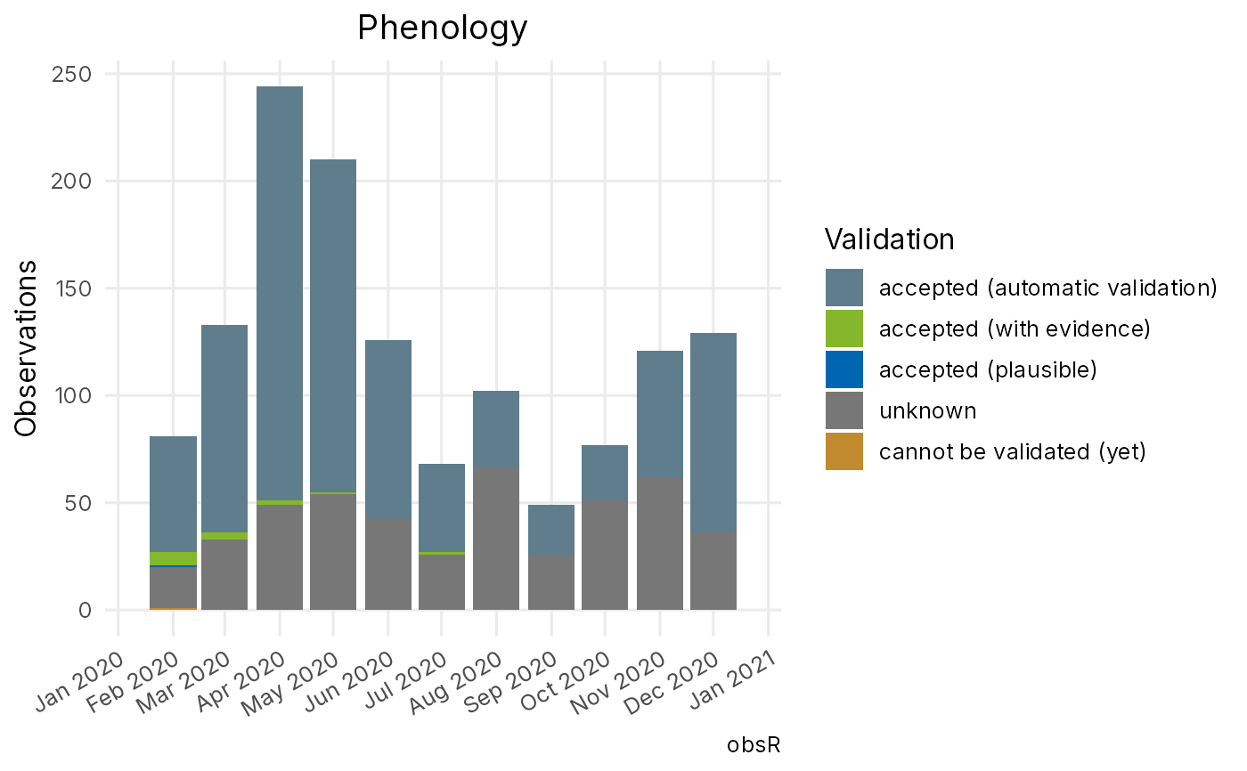
Quick ggplot2 charts over an obs_df (or a path passed to obs_read()). Designed for README captures and first-look exploration, not publication layouts.

Usage

obs_plot(
  data,
  type = c("validation", "phenology", "species", "activity", "sex", "life_stage"),
  top_n = 12,
  ...
)

Arguments

data

An obs_df, a data frame, or a path to an export.

type

One of: "validation" (bar of statuses, official colours), "phenology" (counts by month, stacked by validation), "species" (most frequent taxa), "activity", "sex" (M/F/U colours, individuals), "life_stage" (individuals). Mixed-count SQLite rows are expanded for "sex", "activity" and "life_stage"; see obs_expand(). Maps should use the compact table.

top_n

For "species", "activity" and "life_stage", how many levels to keep.

...

Passed to obs_read() when data is a file path.

Value

A ggplot object.

Font and typography

ggplot2 does not ship a typeface. When the systemfonts package is installed, obsR registers a bundled Inter file so maps and plots look the same on every machine. Without it, the device default sans is used (Arial, Helvetica or DejaVu, depending on the OS). An AGG device such as ragg is needed to actually draw the bundled face.

Examples

obs <- obs_read(obs_example_db())
if (requireNamespace("ggplot2", quietly = TRUE)) {
  obs_plot(obs, "validation")
  obs_plot(obs, "phenology")
}
#> Warning: Removed 5 rows containing missing values or values outside the scale range
#> (`geom_bar()`).